


You just read a new study. How much should you update?
Here's what Bayes' Theorem tells you

You just read a new study: A large-scale experiment found that universal basic income (UBI) doesn’t improve physical health. How much should you update your beliefs on how UBI impacts well-being?
The answer is clear in theory. According to Bayes’ Theorem, the number you need is the Bayes factor. Combine the Bayes factor with your prior, and you’re done.
Unfortunately, it’s hard to apply this recipe in practice. A key reason is that it’s challenging to estimate the size of the Bayes factor.
In this post, I’ll discuss how that can be done. I’ll focus on social science research, as that’s the field I’m most familiar with. After reading this essay, you’ll be able to guesstimate Bayes factors and become a better Bayesian—which, let’s be real, is all anyone could ever wish for.
Here’s what we’ll find:
A quick warning: Estimating Bayes factors is, uhm, an inexact science. The estimates won’t be accurate to three significant digits, and they will depend on some hard-to-check assumptions. Please don’t send me to Science Jail for that.
I. Bayes’ Theorem revisited
Let’s first recap Bayes’ Theorem in its odds form.1
Suppose we have two mutually exclusive hypotheses H₀ and H₁. Bayes’ Theorem states that, after seeing some data D, the posterior odds are
Therefore, to calculate the posterior odds just multiply the prior odds by the Bayes factor. Intuitively, the Bayes factor tells us how many times more likely it is to see the data under the hypothesis H₁ relative to H₀.
For some intuition, let’s work through an example. Let H₁ stand for “UBI improves health” and H₀ for “UBI doesn’t improve health.” Suppose your prior probability that UBI improves health is 75%. You believe that the study, which didn’t find an effect, has a Bayes factor of 0.2 for null findings (i.e., it would be 5x more likely to obtain a null finding if UBI didn’t improve health). What’s your posterior?
Your prior probability is P(H₁) = 0.75, which means that the prior odds (H₁ vs H₀) are 0.75 / (1 – 0.75) = 3.
Multiply the prior by the Bayes factor to obtain the posterior odds: 3 * 0.2 = 0.6.
Finally, convert back from the posterior odds to find the posterior probability: P(H₁ | D) = 0.6 / (0.6 + 1) ≈ 38%.
With these numbers, the study shifts your belief that UBI improves health from 75% to 38%.
II. Calculating the Bayes factor
The calculation above hinges on the size of the Bayes factor. Is a Bayes factor of 0.2 at all reasonable?
We’ll need some math to figure this out. First, some notation:
Denote by p the prior probability that there is an effect (e.g., UBI improves health);
Denote by α the type-I error rate, i.e., the probability of finding an effect, conditional on there being no effect;
Denote by β the type-II error rate, i.e., the probability of not finding an effect, conditional on there being an effect.
We can now draw the potential outcomes in a probability tree:
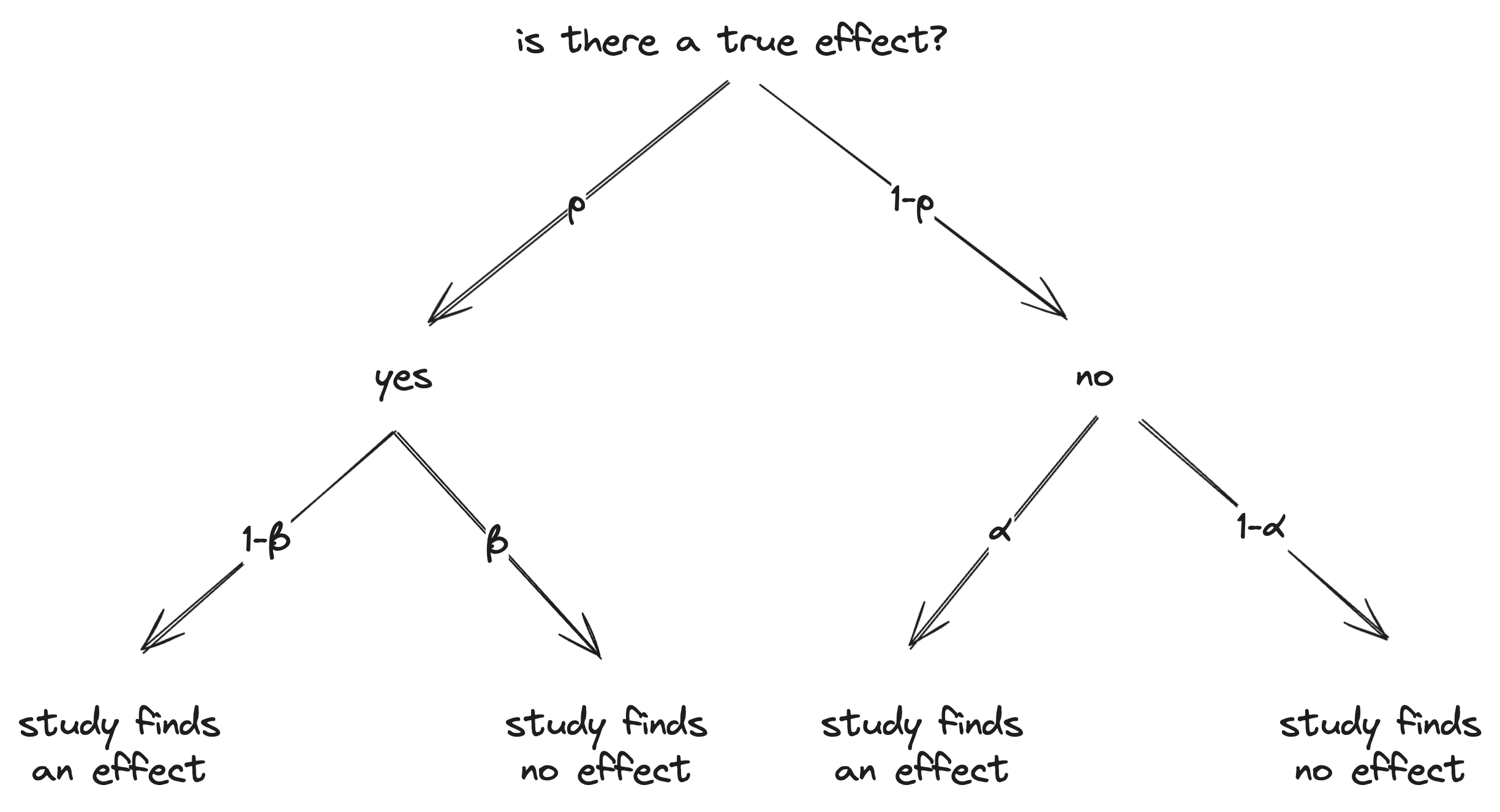
From this tree, we calculate the Bayes factors:
The Bayes factor is a simple function of the type-I and type-II error rates.
For an illustration, suppose that β = 0.20 and α = 0.05 (we’ll see below when these numbers are reasonable). In that case:
After finding an effect, the Bayes factor is (1 – 0.20) / 0.05 = 16;
After finding no effect, the Bayes factor equals 0.20 / (1 – 0.05) ≈ 0.21.
III. Type-I and type-II errors in the wild
We’re making progress, but these formulas only push the question one layer down. How large are type-I and type-II error rates in reality?
Let’s begin with type-I error rates. In classical statistics, tests are designed to achieve a pre-specified type-I error rate. That number is typically 5% or 1%.
Unfortunately, for various reasons, the actual type-I error rate is often much higher than that:
Multiple testing. If a researcher tests many hypotheses, the actual type-I error rate will be inflated. For example, if you test 5 independent hypotheses (each with α = 0.05) but only report positive findings, the combined type-I error is roughly 23%. More generally, there are many choices that researchers can make, from sample definitions to feature engineering, that can inflate the type-I error rate;
Publication bias. Positive research findings are much more likely to be published. This incentivizes researchers to search for positive findings (e.g., via testing multiple hypotheses), again inflating type-I error rates;
Fraud. Unfortunately, some research is outright fraudulent, so we should probably add a few percentage points to allow for the possibility that some data points were fraudulently deleted, adjusted, or just totally made up;
Other errors. Issues such as coding errors could also lead to spurious findings. Systematic research on reproducibility in economics suggests that a large fraction of empirical papers in economics cannot be reproduced.
The upshot is that, even if the nominal type-I error is 1%, the actual error rate is likely substantially higher.
Systematic replication studies confirm this intuition. A large-scale replication effort in psychology found that only around half of studies replicate, while a systematic replication study in economics obtained replication rates of 60–70%. These findings point in the direction of double-digit type-I error rates.
Based on these observations, the numbers below seem like reasonable guesstimates for social science research:
Here, “observational” stands for observational studies, which we’d expect to have higher type-I error rates than experiments.
What about type-II error rates? In experimental research, it’s customary to design studies to achieve 80% statistical power (with statistical power defined as 1 – β). Therefore, β = 0.20 is a sensible estimate of type-II error rates for high-quality experiments.
Unfortunately, as with type-I errors, the actual error rate is likely substantially higher. The major reasons include:
Low sample sizes. The key determinant of statistical power is the sample size. In general, the smaller the sample size, the higher the type-II error rate. If we collect a smaller sample than anticipated (e.g., some participants drop out unexpectedly), we will fail to reach the original statistical power;
Small effect sizes. If the effect we’re trying to estimate is small, we’ll have lower statistical power to detect it. If an experiment was designed to achieve 80% statistical power to detect a large effect, but the actual effect size is smaller, then the actual statistical power is less than 80%;
Measurement error. If variables are measured with error, that leads to an attenuation bias, reducing estimated effect sizes and negatively impacting statistical power;
Other errors. As with type-I errors, multiple other reasons could lead a researcher to fail to detect an effect (e.g., coding errors).
Again, systematic research finds that statistical power is usually substantially lower than the best-practice target of 80%. For example, a recent study by John Ioannidis and co-authors estimates that the median statistical power in published economics research is less than 20%. Similarly, a recent meta-analysis in psychology has found that published studies have a power of only around 20% to detect small effect sizes.
Combining these factors, here are my guesstimates for type-II error rates in social science research:
IV. Bayes factors: Estimates
We can now combine the previous estimates of type-I and type-II error rates to calculate Bayes factors under different scenarios:
You can find the underlying calculations and the estimates at different values of type-I and type-II error rates in this Google Sheet.
Here are the key takeaways:
Bayes factors vary substantially across different scenarios, ranging from 2 to 90 for positive findings. The quality of the study matters a great deal for how much you should update after reading it;
For high-quality experiments, beliefs should move a lot. For example, in the “gold-standard experiment” scenario, the Bayes factor is 90 for positive findings. This finding supports the common intuition that high-quality experimental research is extremely informative;
For medium- and high-quality observational studies, estimated Bayes factors are between 2 and 6 for positive findings, and 0.4 to 0.8 for null findings, which is notably lower than in experimental work;
For low-quality studies, you may get a Bayes factor with the “wrong magnitude,” such as a Bayes factor of less than 1 for positive findings. The reason is that, with very high type-I error rates, we attribute a positive finding to a false positive, reducing our confidence in a true effect.
V. Conclusions and caveats
Let’s return to our original question: How much should you update your beliefs on UBI after reading that new study?
After reading the paper and its pre-analysis plan, I would classify the study as a “high-quality experiment.” As the study didn’t find an effect, the table above suggests using a Bayes factor of 0.21. You can combine that with your prior for the updated beliefs.
My own prior is that most interventions don’t have a positive impact. Hence, I’d start with a prior probability of around 25%. Combining that with the Bayes factor of 0.21 results in a posterior probability of roughly 7%. That’s pretty bad news for UBI as a health-policy tool.
Before concluding, I want to highlight a few caveats:
The model in this post has a strict “there is a true effect” vs “there is no true effect” distinction. In reality, things are not so binary, and it’s helpful to think of a distribution of potential effect sizes. The current model is not very well-suited for that;2
The estimated Bayes factors are only as good as the estimated type-I and type-II error rates. If you disagree with some of the assumptions I made, feel free to plug in your preferred numbers or look up the Bayes factors at different error rates in the spreadsheet;
None of what I presented here seems like it should be novel, but I haven’t come across it before in this specific form. If I’m missing some key literature references, my apologies.
Finally, there’s a deeper philosophical question. Can you really do a full Bayesian update in practice? The world is a complicated place, and maybe the best we can do is draw some qualitative insights from the math (like, “update more on higher-quality experiments”), and call it a day.
I’m a bit of an idealist here. I believe you can do quantitative Bayesian updating in the real world, though not to an extreme level of precision. In practice, I don’t think we can judge whether the right Bayes factor is 2.00 or 2.25 with any degree of confidence. But a quick, back-of-the-envelope, orders-of-magnitude Bayesian calculation? I think that’s possible and helpful. Putting probabilities on things is great, for many reasons.
Whatever your philosophical stance, though, if you need to update quantitatively on research findings, I hope this post brings some clarity.
Happy updating!
If you want to learn more about Bayes’ Theorem and get practice with the odds form, this episode of 80,000 Hours is a great practical intro.
You can get around this a bit by re-interpreting β as the “type-II error rate for an effect of a given size, e.g., a moderate effect.”